Examples

This page provides practical examples demonstrating common use cases with real code from the package.

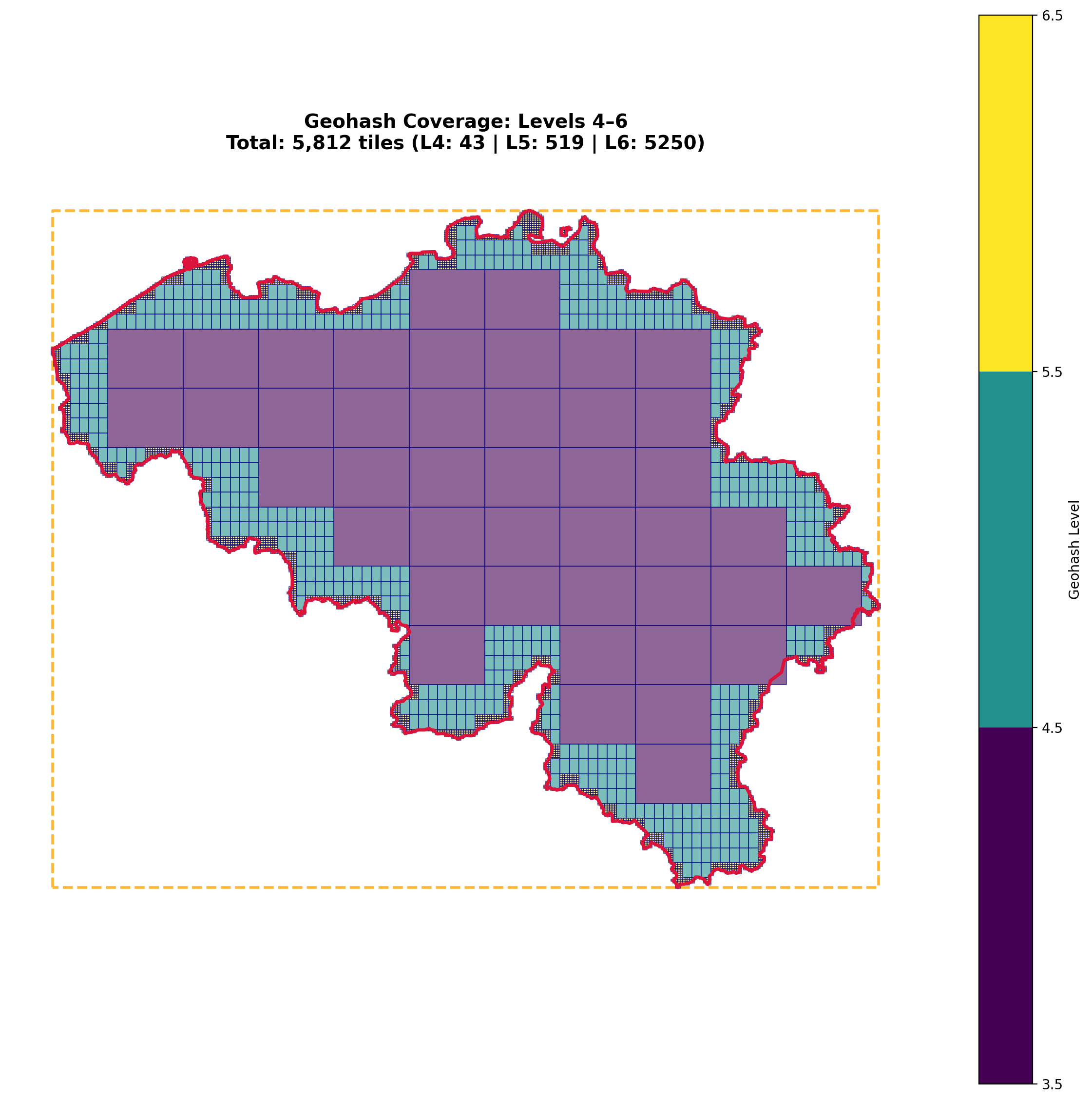
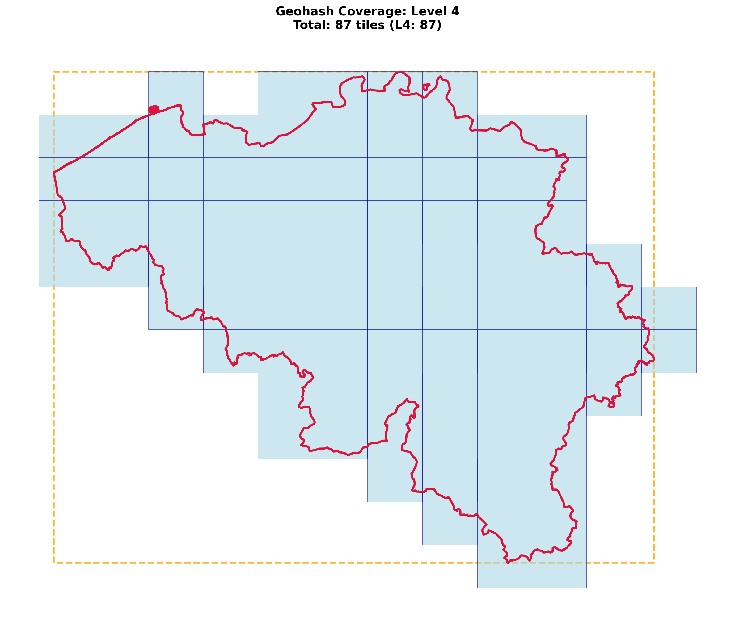
Basic Example: Adaptive and Single-Level Coverage

Download a country and generate both adaptive and single-level geohash coverage:

from shapely import MultiPolygon, Polygon
from sigmap.polygeohasher import download_gadm_country, build_single_multipolygon, \
    adaptive_geohash_coverage, plot_geohash_coverage, geohash_coverage
from sigmap.polygeohasher.plot_geohash_coverage import plot_level_statistics

# Download Belgium
country_gdf = download_gadm_country("BEL", cache_dir='./gadm_cache')

# Build geometry
country_geom = build_single_multipolygon(country_gdf)

# Generate adaptive coverage
geohash_dict, tiles_gdf = adaptive_geohash_coverage(country_geom, 2, 6)

# Plot the adaptive coverage map
plot_geohash_coverage(
    country_geom, geohash_dict, tiles_gdf,
    style='adaptive',
    save_path='./generated_plot/adaptive_coverage.png',
)

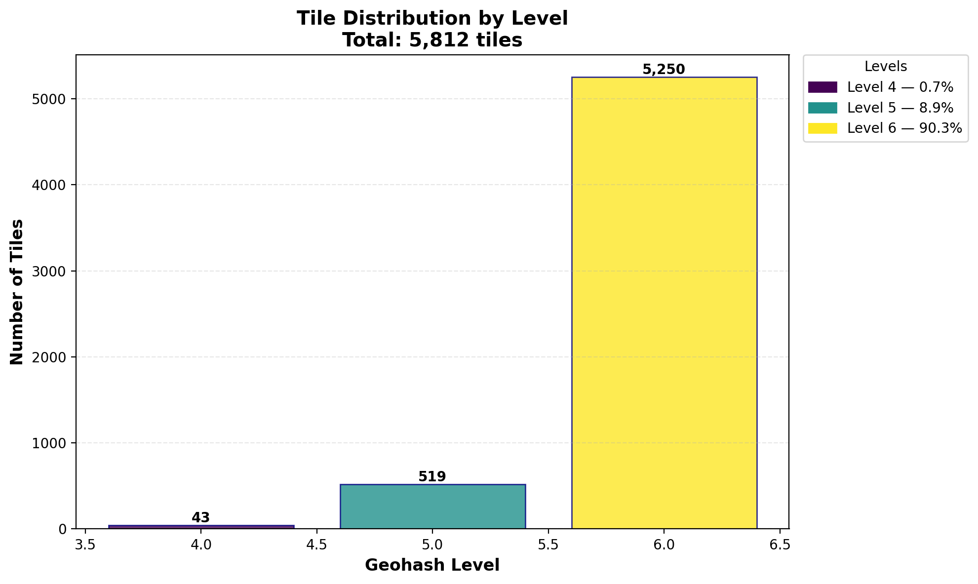
# Plot tile repartition statistics
plot_level_statistics(
    geohash_dict,
    style='bar',
    save_path='./generated_plot/level_stats_bar.png'
)
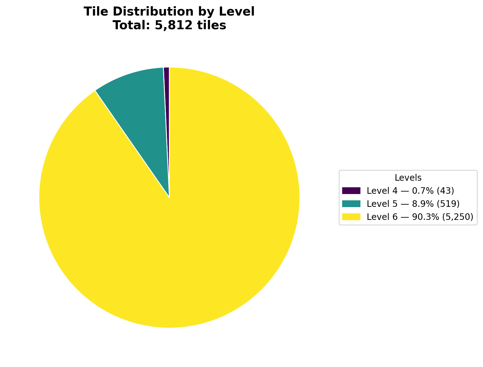
plot_level_statistics(
    geohash_dict,
    style='pie',
    save_path='./generated_plot/level_stats_pie.png'
)

# Generate single-level coverage
geohash_dict_single = geohash_coverage(country_geom, level=4)

# Plot single-level coverage
plot_geohash_coverage(
    country_geom, geohash_dict_single,
    style='single',
    save_path='./generated_plot/single_coverage.png',
)

Result:

Statistics:

Comparing Coverage Types

Count tiles per coverage type for both adaptive and single-level:

from sigmap.polygeohasher import download_gadm_country, build_single_multipolygon, \
    adaptive_geohash_coverage, geohash_coverage

def counting_tiles_per_coverage(geom, min_level, max_level):
    # Adaptive coverage from min to max
    geohash_dict, tiles_gdf = adaptive_geohash_coverage(
        geom,
        min_level=min_level,
        max_level=max_level,
        use_strtree=True,
    )

    print("=== MIN-MAX LEVEL RESULTS ===")
    for key in sorted(geohash_dict.keys()):
        print(f"Level {key}: {len(geohash_dict[key])} tiles")
    print(f"Total tiles: {sum(len(v) for v in geohash_dict.values())}")

    # Single level
    geohash_dict_single_level = geohash_coverage(
        geom,
        level=2,
        use_strtree=True,
        debug=True
    )

    print("\n=== SINGLE LEVEL RESULTS ===")
    for key in sorted(geohash_dict_single_level.keys()):
        print(f"Level {key}: {len(geohash_dict_single_level[key])} tiles")

# Use with country
ISO3 = "BEL"
MIN_LEVEL = 2
MAX_LEVEL = 5
CACHE_DIR = './gadm_cache'

country_dataframe = download_gadm_country(ISO3, cache_dir=CACHE_DIR)
country_geometry = build_single_multipolygon(country_dataframe)
counting_tiles_per_coverage(country_geometry, MIN_LEVEL, MAX_LEVEL)

Working with Geohash Conversions

Convert geohashes to boxes and MultiPolygons:

from sigmap.polygeohasher.utils.geohash import (
    geohashes_to_boxes,
    geohashes_to_multipolygon,
    get_geohash_children
)

# Single geohash to box
geohash = "u4pruyd"
boxes = geohashes_to_boxes(geohash)
print(f"Geohash: {geohash}")
print(f"Box polygon: {boxes[geohash]}")
print(f"Bounds (lon_min, lat_min, lon_max, lat_max): {boxes[geohash].bounds}")
print(f"Area: {boxes[geohash].area:.10f} square degrees")

# Multiple geohashes to boxes
geohashes = ["u4pru", "u4prv", "u4prw", "u4pry"]
boxes = geohashes_to_boxes(geohashes)
print(f"\nNumber of geohashes: {len(geohashes)}")
print(f"Number of boxes: {len(boxes)}")
for gh, box in boxes.items():
    print(f"  {gh}: bounds = {box.bounds}")

# Get children geohashes
parent = "u4pr"
children = get_geohash_children(parent)[:8]  # First 8 children
print(f"\nParent geohash: {parent}")
print(f"Children: {children}")

# Create dissolved MultiPolygon
multi_poly = geohashes_to_multipolygon(children, dissolve=True)
print(f"\nResult type: {type(multi_poly).__name__}")
print(f"Number of polygons: {len(multi_poly.geoms) if hasattr(multi_poly, 'geoms') else 1}")
print(f"Total area: {multi_poly.area:.10f} square degrees")

Visualizing Boxes vs MultiPolygons

Compare individual boxes with dissolved and separate MultiPolygons:

import matplotlib.pyplot as plt
import geopandas as gpd
from sigmap.polygeohasher.utils.geohash import (
    geohashes_to_boxes,
    geohashes_to_multipolygon
)

# Create some geohashes
geohashes = ["u0gnu", "u0gnv", "u0gnw", "u0gny",
             "u0gnz", "u0gnx", "u0gnq", "u0gnm"]

# Get boxes
boxes = geohashes_to_boxes(geohashes)

# Create MultiPolygons (dissolved and separate)
multi_poly_dissolved = geohashes_to_multipolygon(geohashes, dissolve=True)
multi_poly_separate = geohashes_to_multipolygon(geohashes, dissolve=False)

# Create plot
fig, axes = plt.subplots(1, 3, figsize=(18, 6))

# Plot 1: Individual boxes
gdf1 = gpd.GeoDataFrame({'geohash': list(boxes.keys())},
                        geometry=list(boxes.values()), crs='EPSG:4326')
gdf1.plot(ax=axes[0], facecolor='lightblue', edgecolor='navy', alpha=0.6)
axes[0].set_title(f'Individual Boxes\n{len(boxes)} separate polygons', fontweight='bold')
axes[0].set_axis_off()

# Plot 2: Separate MultiPolygon
gdf2 = gpd.GeoDataFrame({'geometry': [multi_poly_separate]}, crs='EPSG:4326')
gdf2.plot(ax=axes[1], facecolor='lightgreen', edgecolor='darkgreen', alpha=0.6)
axes[1].set_title(f'MultiPolygon (Separate)\n{len(multi_poly_separate.geoms)} polygons',
                  fontweight='bold')
axes[1].set_axis_off()

# Plot 3: Dissolved MultiPolygon
gdf3 = gpd.GeoDataFrame({'geometry': [multi_poly_dissolved]}, crs='EPSG:4326')
gdf3.plot(ax=axes[2], facecolor='lightcoral', edgecolor='darkred', alpha=0.6)
n_polys = len(multi_poly_dissolved.geoms) if hasattr(multi_poly_dissolved, 'geoms') else 1
axes[2].set_title(f'MultiPolygon (Dissolved)\n{n_polys} polygon(s)', fontweight='bold')
axes[2].set_axis_off()

plt.tight_layout()
plt.savefig('./generated_plot/geohash_boxes_comparison.png', dpi=200, bbox_inches='tight')
plt.close()

Result:

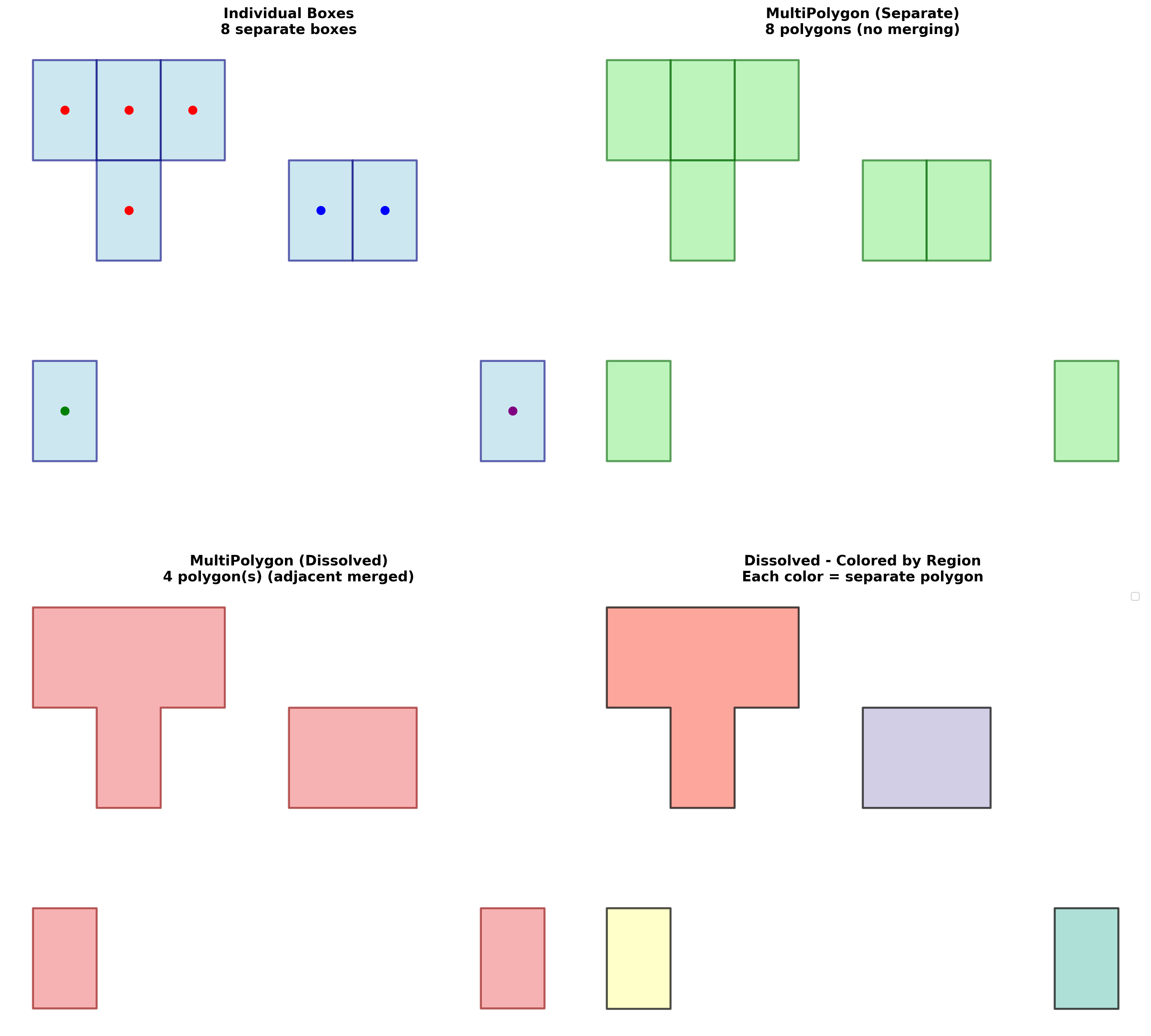
Working with Isolated Polygons

Visualize how dissolved MultiPolygons handle isolated (disjoint) polygons:

import matplotlib.pyplot as plt
import geopandas as gpd
from sigmap.polygeohasher.utils.geohash import (
    geohashes_to_boxes,
    geohashes_to_multipolygon
)

# Create geohashes with distinct groups:
# Group 1: Adjacent tiles (will merge when dissolved)
group1 = ["u0gnb", "u0gnc", "u0gnf", "u0gn9"]
# Group 2: Adjacent tiles in different location
group2 = ["u0gns", "u0gnt"]
# Group 3 & 4: Isolated tiles
group3 = ["u0gn0"]
group4 = ["u0gnp"]

all_geohashes = group1 + group2 + group3 + group4

# Get boxes
boxes = geohashes_to_boxes(all_geohashes)

# Create MultiPolygons
multi_poly_separate = geohashes_to_multipolygon(all_geohashes, dissolve=False)
multi_poly_dissolved = geohashes_to_multipolygon(all_geohashes, dissolve=True)

# Create visualization
fig, axes = plt.subplots(2, 2, figsize=(16, 16))

# Plot individual boxes
gdf1 = gpd.GeoDataFrame({'geohash': list(boxes.keys())},
                        geometry=list(boxes.values()), crs='EPSG:4326')
gdf1.plot(ax=axes[0, 0], facecolor='lightblue', edgecolor='navy', alpha=0.6, linewidth=2)
axes[0, 0].set_title(f'Individual Boxes\n{len(boxes)} separate boxes',
                     fontweight='bold', fontsize=14)
axes[0, 0].set_axis_off()

# Plot separate MultiPolygon
gdf2 = gpd.GeoDataFrame({'geometry': [multi_poly_separate]}, crs='EPSG:4326')
gdf2.plot(ax=axes[0, 1], facecolor='lightgreen', edgecolor='darkgreen',
          alpha=0.6, linewidth=2)
axes[0, 1].set_title(f'MultiPolygon (Separate)\n{len(multi_poly_separate.geoms)} polygons',
                     fontweight='bold', fontsize=14)
axes[0, 1].set_axis_off()

# Plot dissolved MultiPolygon
gdf3 = gpd.GeoDataFrame({'geometry': [multi_poly_dissolved]}, crs='EPSG:4326')
gdf3.plot(ax=axes[1, 0], facecolor='lightcoral', edgecolor='darkred',
          alpha=0.6, linewidth=2)
n_polys = len(multi_poly_dissolved.geoms) if hasattr(multi_poly_dissolved, 'geoms') else 1
axes[1, 0].set_title(f'MultiPolygon (Dissolved)\n{n_polys} polygon(s)',
                     fontweight='bold', fontsize=14)
axes[1, 0].set_axis_off()

# Plot dissolved with different colors per polygon
if hasattr(multi_poly_dissolved, 'geoms'):
    colors = plt.cm.Set3(range(len(multi_poly_dissolved.geoms)))
    for i, (geom, color) in enumerate(zip(multi_poly_dissolved.geoms, colors)):
        gdf_part = gpd.GeoDataFrame({'id': [i]}, geometry=[geom], crs='EPSG:4326')
        gdf_part.plot(ax=axes[1, 1], facecolor=color, edgecolor='black',
                      alpha=0.7, linewidth=2, label=f'Region {i + 1}')
    axes[1, 1].legend(loc='upper right', fontsize=10)

axes[1, 1].set_title(f'Dissolved - Colored by Region',
                     fontweight='bold', fontsize=14)
axes[1, 1].set_axis_off()

plt.tight_layout()
plt.savefig('./generated_plot/geohash_isolated_polygons.png', dpi=200, bbox_inches='tight')
plt.close()

Result:

Full Workflow: Coverage to MultiPolygon

Complete workflow from downloading a country to creating a MultiPolygon from coverage:

from sigmap.polygeohasher.utils.gadm_download import download_gadm_country
from sigmap.polygeohasher.utils.geohash import geohashes_to_multipolygon
from sigmap.polygeohasher.utils.polygons import build_single_multipolygon
from sigmap.polygeohasher.adaptative_geohash_coverage import geohash_coverage

# Load country
country_gdf = download_gadm_country("LUX", cache_dir='./gadm_cache')
country_geom = build_single_multipolygon(country_gdf)

# Generate coverage
geohash_dict = geohash_coverage(country_geom, level=5)

# Extract geohashes
all_geohashes = []
for level, geohashes in geohash_dict.items():
    all_geohashes.extend(geohashes)

print(f"Generated {len(all_geohashes)} geohashes for Luxembourg (level 5)")

# Convert to MultiPolygon
coverage_polygon = geohashes_to_multipolygon(all_geohashes, dissolve=True)

print(f"\nCoverage polygon:")
print(f"  Type: {type(coverage_polygon).__name__}")
print(f"  Area: {coverage_polygon.area:.6f} square degrees")
print(f"  Bounds: {coverage_polygon.bounds}")

# Compare with original country
print(f"\nOriginal country:")
print(f"  Area: {country_geom.area:.6f} square degrees")
print(f"  Coverage ratio: {(coverage_polygon.area / country_geom.area * 100):.2f}%")

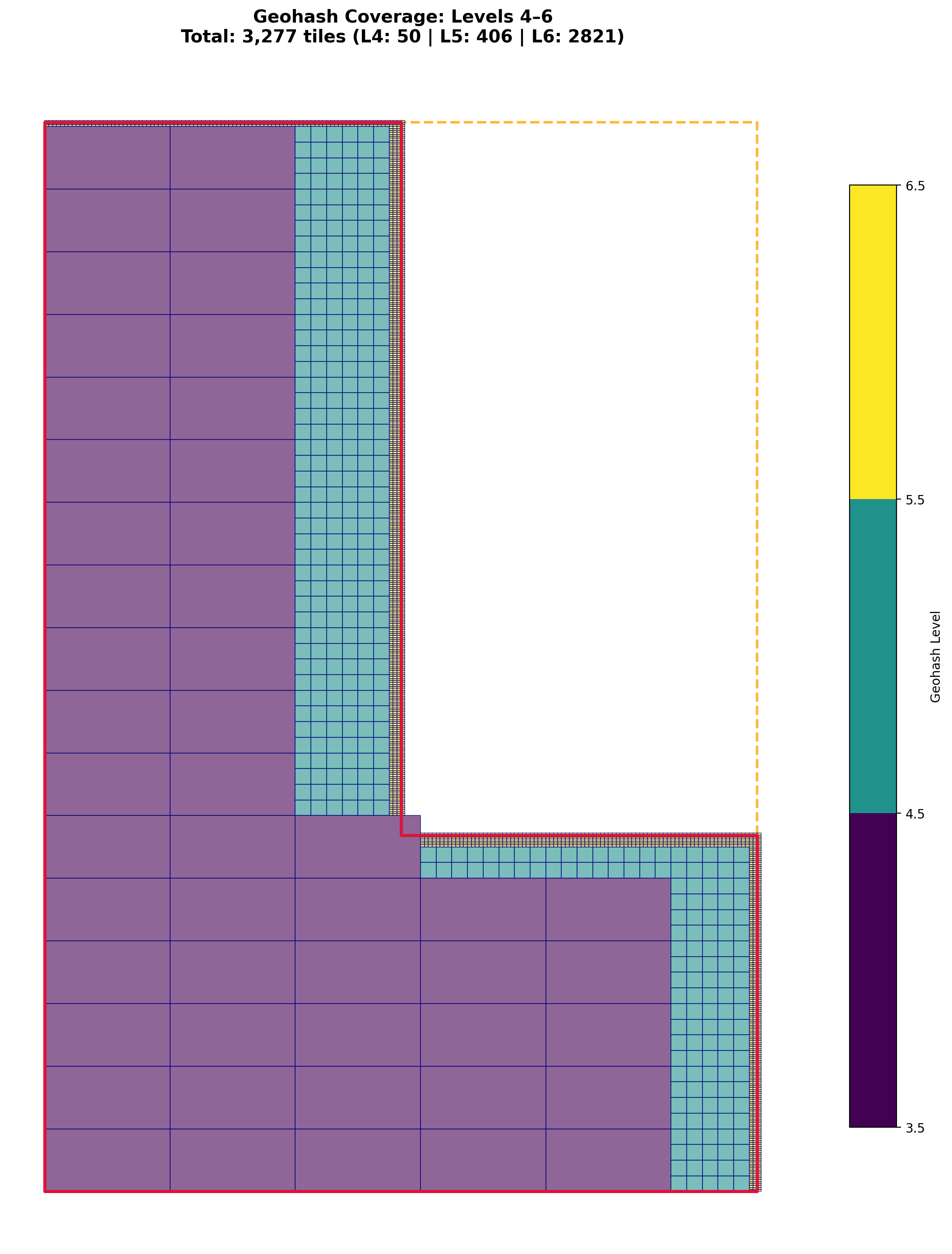
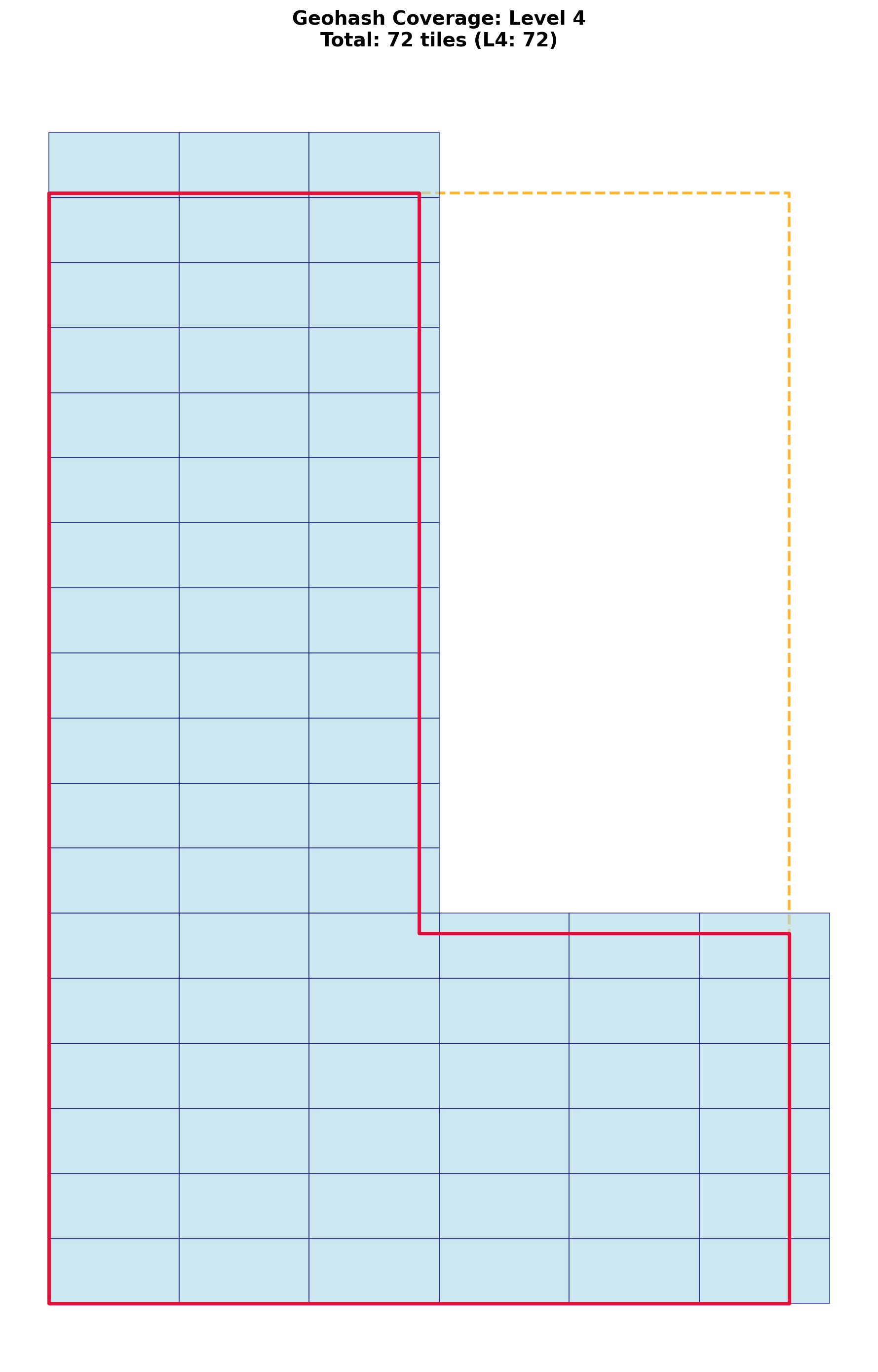
Custom Polygon Example

Work with custom polygons (not just countries):

from shapely import Polygon
from sigmap.polygeohasher import adaptive_geohash_coverage, plot_geohash_coverage

def custom_polygon_creation() -> Polygon:
    # L-shaped polygon
    vertex = [
        (0, 0), (2, 0), (2, 1), (1, 1),
        (1, 3), (0, 3), (0, 0)
    ]
    return Polygon(vertex)

custom_geom = custom_polygon_creation()

# Generate adaptive coverage
geohash_dict, tiles_gdf = adaptive_geohash_coverage(custom_geom, 2, 6)

# Plot with custom save path
plot_geohash_coverage(
    custom_geom, geohash_dict, tiles_gdf,
    style='adaptive',
    save_path='./generated_plot/CUSTOM_adaptive_coverage.png',
)

# Note: You can see on the inside corner of the L-shape a tile with a corner off the polygon.
# This is due to the default threshold (95%) - tiles are considered "fully contained" if
# (1 - area_outside/area_total) >= threshold.
# To avoid this, set coverage_threshold=1.0:
# geohash_dict, tiles_gdf = adaptive_geohash_coverage(
#     custom_geom, 2, 6, coverage_threshold=1.0
# )

Result: